5/11 Phasors: Passive RL Circuit Response

Today, we talked about sinusoids and phasors.
A sinusoid is a signal that has the form of the sine or cosine function.

where
Vm = the amplitude of the sinusoid
ω = the angular frequency in radians/s
ωt = the argument of the sinusoid

A sinusoid can be expressed in either sine of cosine form. With these identities, it is easy to express both as either sine or cosine with positive amplitudes.

By using these relationships, we can transform a sinusoid from sine form to cosine form or vice versa.
The picture below is the graphical approach.

To add A cos ωt and B sin ωt, we note that A is the magnitude of cos ωt while B is the magnitude of sin ωt.
The magnitude and argument of the resultant sinusoid in cosine form is readily obtained from the triangle.


Next, we talked about phasors, which are more convenient than sinusoids to work with sine and cosine functions.
A phasor is a complex number that represents the amplitude and phase of a sinusoid.


To deal with the complex numbers calculations, the following operations are important.

We did a little example of how to transform rectangular form to polar form.

Also, we did a example of the calculation of polar form.

Next, we introduced how to determine which one the leading direction and lagging direction are.

Then, we did a example of two sinusoids function addition.


The derivative v(t) is transformed to the phasor domain as jωV
The integral of v(t) is transformed to the phasor domain as V/jω
These are useful in finding the steady-state solution, which does not require knowing the initial values of the variable involved.
The picture below is the example of the transformation of the derivative of v(t) and the integral of v(t) to the phasor domain.

The table below summarizes the time-domain and phasor-domain representations of the circuit elements.

Then, we did lab.

Phasors: Passive RL Circuit Response
Pre-lab

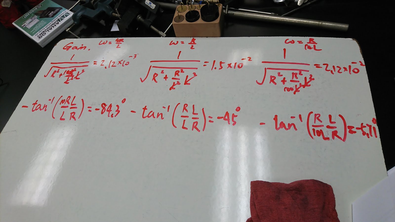
The picture above is the amplitude gain and phase difference between the input voltage and the input current with different frequency.

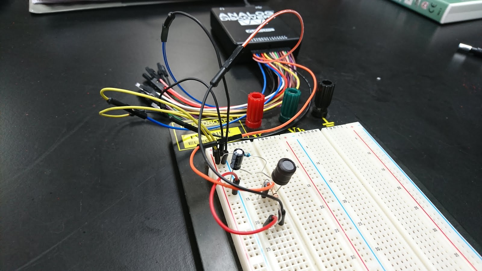
The picture below is the basic set up for this lab.


Result:

With the cutoff frequency, the phase difference is (16.87)/(135)*360 = -44.9degree, and the gain is 13.28/668.3 = 0.01987


With ten times the cutoff frequency, the phase difference is (3.102)/(13.5)*360 = -82.72degree, and the gain is 2.155(mA)/223.2(mV) = 0.009655


With one tenth of cutoff frequency, the phase difference is (0.03)/1.45 = -7.448degree, and the gain is 0.001675/1.013 = 0.0016535


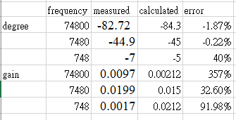
The picture above is the comparison of experimental and theoretical data.
From the data, we can see that we successfully finished the lab, especially on the phase difference.

Summary

We learned about sinusoids and phasors, which are different ways to deal with AC circuit. Also, we learned how to determine the phase difference and gain according to the graph. By comparing the data, we can see the experiment matched what we expected.

5/9 RLC Circuit Response

Today, we talked about Schmitt Trigger, whihc is a logic input type that provides hysteresis or two different threshold voltage levels for rising and falling edge. This is useful because it can avoid the errors when we have noisy input signals from which we want to get square wave signals. (From Day 19 2nd Order Circuits Contc.pdf)
The picture below is what the operational amplifier based schmitt trigger looks like:

Next, we introduced the non-symmetrical schmitt trigger.

The picture below is what the the non-symmetrical schmitt trigger looks like.

Then, we talked about the step response of a series and parallel RLC circuit.

Review questions:

Next, we did lab.

RLC Circuit Response

Pre-lab

The picture is the differential equation relating Vin and Vout for the system.

By using the equation, we can determine the damping ratio and natural frequency of the circuit.

The damping ratio is 1563.8 and natural frequency is 10105.8Hz.

The picture below is the basic set up for this lab.

Result:

The damping ratio from the graph is 0.25, rise time is 2.15*10^-4, DC gain is 8.

After lab, we talked more about the second order circuits.

Summary

We learned about what the Schmitt Trigger is, and reviewed about RLC circuit which is second order circuit.  In order to recover the transmitted analog

signal, the output is smoothed by letting it pass through a “smoothing” circuit, as illustrated at right. An RLC circuit may be used as the smoothing circuit.

5/2 Series RLC Circuit Step Response

Before, we considered the circuits with only one element (a capacitor or a inductor), and the circuits are first-order.
Today, we talked about the circuits with two storage elements which is known as second-order circuits because their responses are described by differential equations that contain second derivatives.
The main idea of this kind of problems is to get the value of  v(0), i(0), dv(0)/dt, di(0)/dt, i( ∞ ), and v( ∞ ). By determining these value, we can solve the problems easily.
Next, we talked about the source free series RLC circuit.
 
By determining  α  and ωo, we can see what type of this circuit is.
1. If α > ω 0 , we have the overdamped case.
2. If α = ω 0 , we have the critically damped case.
3. If α < ω 0 , we have the underdamped case.
We did a example of the source free series RLC circuit.


Series RLC Circuit Step Response
Pre-lab

This is the prediction of differential equation, damping ratio, natural frequency, and damped natural frequency of this lab.

The picture below is the basic set up for this lab.

The graph below is the result for this lab.

The  rise time of the graph is 1.241ms.
The overshoot is 3.5ms.
The oscillation frequency is 23485Hz.
Out estimated damping ratio, natural frequency and damped natural frequency is in the pre-lab.
Our estimated DC gain is 2.383 (in the beginning of the transient).

Summary

From today's lecture, we learned the source free series RLC circuit and the source free parallel RLC circuit. By determining α and ω 0 , we can determine which case the circuit is. From the lab, we learned how to determine the rise time, overshoot time, and the oscillation frequency. And from the graph, we can see that there is a sudden change when we apply the voltage to the circuit. An automobile ignition system takes advantage of this feature. By creating a large voltage (thousands of volts) between the electrodes, a spark is formed across the air gap, thereby igniting the fuel.