6/8 Passive RL Filter

Today is the last day of the lecture.
We talked about filters. A filter is a circuit that is designed to pass signals with desired frequencies and reject or attenuate others. (From Day 27 Filters.pdf)
A filter can be used to limit the frequency spectrum of a signal to some
specified band of frequencies.
There are two kinds of filters: passive and active filters.
A filter is a passive filter if it consists of only passive elements R, L, and C.
A filter is an active filter if it consists of active elements (such as transistors and op amps) in addition to passive elements R, L, and C.
The picture shows the differences between four types of filters.

Low pass filter will pass low frequency (C in RC Series or R in RL Series).
High pass filter will pass high frequency (R in RC series).
Band pass filter will pass middle frequency (R in RLC Series).
Band stop filter will pass frequency other than the middle frequency (LC in RLC Series).
We did some example:


Then, we did lab.

Passive RL Filter
Pre-lab

We calculated the cut off frequency, which is 15915Hz.

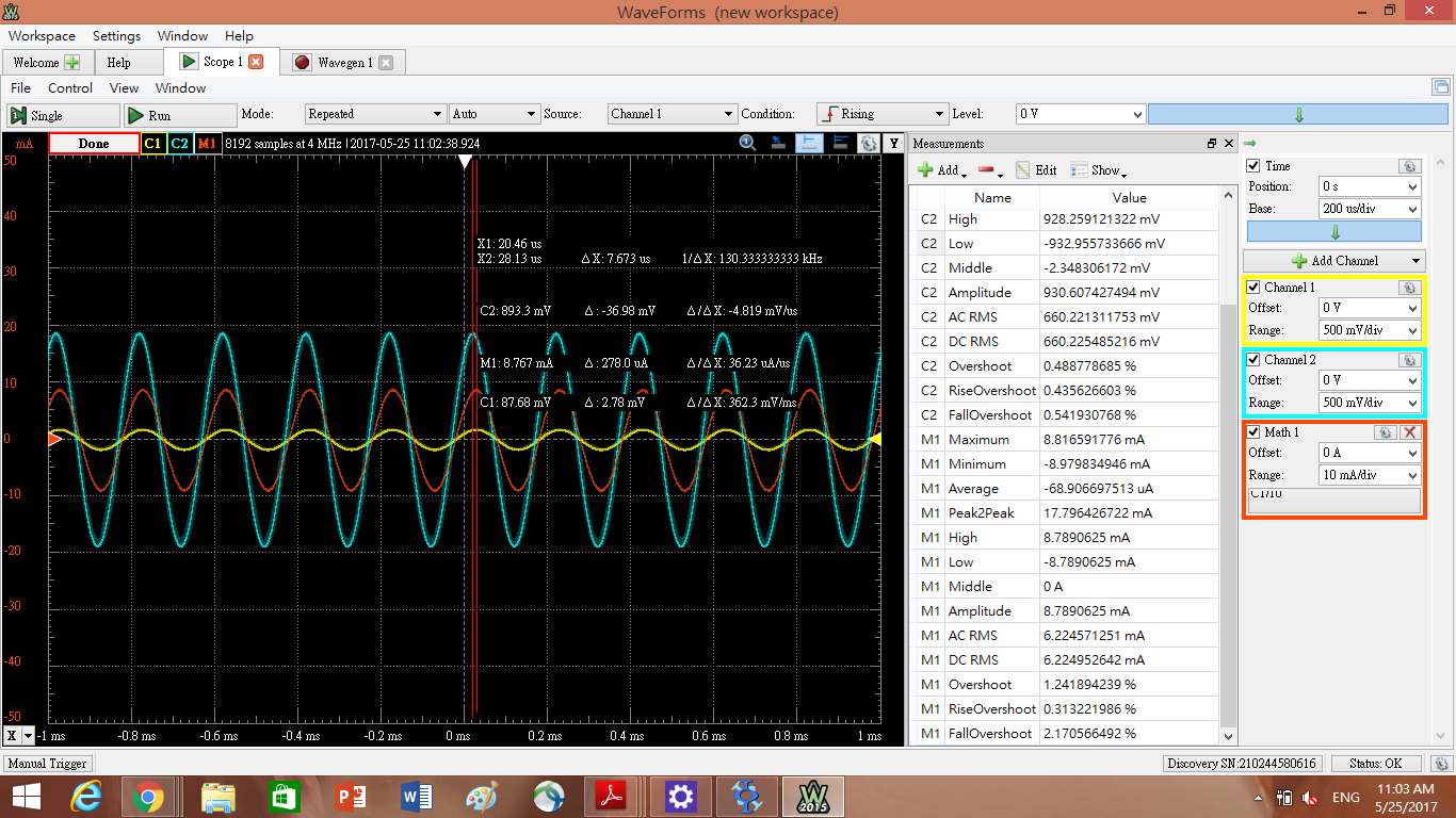
Result:
Before cutoff frequency (Resistor Voltage)


At the cutoff frequency and after:


Before the cutoff voltage:


In and after the cutoff frequency:



The graph below are the the graphs for phase vs frequency and transfer function vs frequency of the voltage output of the resistor.


The graph below are for phase vs frequency and transfer function vs frequency of the voltage output of the inductor.

Summary

Today, we learned the differences between each filters and did a lab of the resistor voltage acting like a low pass filter and the inductor voltage acting like a high pass filter. 

6/6 No Lab. Bode Plots

Today's lecture is about Bode Plots.
Bode plots are semilog plots of the magnitude (in decibels) and phase (in degrees) of a transfer function versus frequency.
(From Day 26 BODE PLOTS.pdf)
H(ω) has seven different factors that can appear in various combinations in a transfer function.

We did a example in the class.

By following the summary of Bode plots for the seven factors, we can easily plot the transfer function.
Here is the summary of Bode plots for the seven factors:

Here is another example of how to plot the graph.


Then, we learned series resonance and parallel resonance.
Resonance is a condition in an RLC circuit in which the capacitive and inductive reactances are equal in magnitude, thereby resulting in a purely resistive impedance.
(From Day 26 BODE PLOTS.pdf)
We introduced a new thing called the quality factor.
The quality factor of a resonant circuit is the ratio of its resonant frequency
to its bandwidth.
The table below shows a summary of the characteristics of the series and parallel resonant circuits:

Summary

We basically practiced how to plot bode plots the entire day, and learned how to determine the transfer function by looking at the bode plot. After a lot of bode plots, we learned resonance which occurs in any circuit that has at least one inductor and one capacitor.

5/30 Signals with Multiple Frequency Components

Before the third exam, we learned frequency dependence, transfer functions, and decibel scale.
The frequency response of a circuit is the variation in its behavior with change in signal frequency, and is also be considered as the variation of the gain and phase with frequency.
The transfer function H(ω) of a circuit is the frequency-dependent ratio of a phasor output Y(ω) (an element voltage or current) to a phasor input X(ω) (source voltage or current).
An easier way to view transfer function is just simply replace all the jω to s.
The transfer function H(ω) can be expressed in terms of its numerator polynomial N(ω) and denominator polynomial D(ω) as

The roots of N(ω) = 0 are called the zeros of H(ω).
The roots of D(ω) = 0 are called the poles of H(ω).
By knowing the value that makes N(ω) = 0 and D(ω) = 0, we can plot the graph of  transfer function.
We did some simple examples of transfer function by using current divider.


Next, we introduced the decibel scale.
Because it is now easy to quickly plot the magnitude and phase of the transfer function, we introduced a more systematic way of obtaining the frequency response--Bode plots.
Two things are important to note from the decibel (dB) equations:
1. That 10 log is used for power, while 20 log is used for voltage or current, because of the square relationship between them (P = V^2/R = I 2 R).
2. That the dB value is a logarithmic measurement of the ratio of one variable to another of the same type. Therefore, it applies in expressing the transfer function H when it is a gain which are dimensionless quantities, but not when it is an impedance
(From Day 25 Frequency Dependencec.pdf)

Then, we did lab.

Signals with Multiple Frequency Components
Pre-lab

The magnitude response (the ratio of the amplitude of the output sinusoid to the input sinusoid) of the circuit at frequencies of 500Hz, 1000Hz, and 10kHz.
As the frequency increases, the voltage gain decreases.

Result:
Use the waveform generator to apply a custom waveform to the circuit.

The yellow line is the output voltage across the resistor, and the blue line is the input voltage of the circuit.
The overall shape is a sine wave forming from a lot of small waves.
A low frequency signal has a bigger magnitude of gain and a high frequency signal has a smaller magnitude of gain.

Use the waveform generator to apply a sinusoidal sweep to the circuit.

The yellow line is the output voltage across the resistor, and the blue line is the input voltage of the circuit.
This graph shows the gain of different frequencies signal from 100Hz to 10kHz.
When the frequency is low, the gain is relatively small, and when the frequency is high, the gain is relatively big.

Summary

The class before the 3rd exam, we learned frequency dependence, transfer functions, and decibel scale. By plotting the the transfer function graph, we can see that how to determine the gain of the circuit. From the lab, we know the relationship between the frequency and the gain.

5/25 Apparent Power and Power Factor

Today, we talked about effective or RMS value, apparent power, power factor, and complex power.
The effective value of a periodic current is the dc current that delivers the same
average power to a resistor as the periodic current.
The effective value of a periodic signal is its root mean square (RMS) value.

The apparent power (in VA) is the product of the RMS values of voltage and current. 

The power factor is the cosine of the phase difference between voltage and current. It is also the cosine of the angle of the load impedance.

Here is the power summary:

The picture below is the relationship between effective value and max value.

We did some example of how we use the equation to find what we want.

Then, we did lab.

Apparent Power and Power Factor

Pre-lab

The picture above is when RL=10ohms.

The table below is what we calculated for different resistance value.

The actual resistor we used are 10.8ohms, 47.1 ohms, and 99.3ohms.

The picture below is the basic set up for this lab.

Result:

RL = 10 ohms

The RMS value of load voltage is 627mV.

The RMS value of load current is 18.7mA.

The phase difference is 64.44 degree.

RL = 47 ohms

The RMS value of load voltage is 625.1mV.

The RMS value of load current is 10.68mA.

The phase difference is 36.83 degree.

RL = 100 ohms

The RMS value of load voltage is 660.1mV.

The RMS value of load current is 6.22mA.

The phase difference is 12.6 degree.

The table below is the comparison of experimental value and calculated value.

From the graph above, we successfully verify the apparent power equation Irms*Vrms = Power, and the power factor is cos(V-I).

Summary

Today, we learned many new things: effective or RMS value, apparent power, power factor, and complex power. By learning these terms, we can deal with power in AC circuit, and know how power is viewed in actual world--the importance of power factor in electricity consumption cost.

5/23 Op Amp Relaxation Oscillator

Today, we continued on the AC circuit analysis with op amp.
First, we did a example of the circuit with op amp with AC voltage supply. (I did not take a picture.)
An oscillator is a circuit that produces an ac waveform as output when powered by a dc input. Oscillator is a device which transform DC signal to AC signal. Without the existence of oscillator, AC signal will not exist.

In order for sine wave oscillators to sustain oscillations, they must meet the Barkhausen criteria:

1. The overall gain of the oscillator must be unity or greater. Therefore, losses must be compensated for by an amplifying device.

2. The overall phase shift (from input to output and back to the input) must be zero.

(From Day 23 AC Op Amps , Oscillators, AC Power.pdf)

Then, we did lab.

Op Amp Relaxation Oscillator

Pre-lab

We were planning to create a signal with the frequency 254 Hz (which is the last 3 digits of my student id). We need to have R=18k to produce this frequency.

The picture above is the basic set up for this lab. We used one 12k ohms resistor and two 3k ohms resistors to produce 18k ohms resistance.

Using Everycircuit, we have successfully proven that the circuit will provide an oscillating signal.

The picture is the result of our lab. Our measured value of frequency in our oscillator is 1/0.003740 = 267.3Hz. Comparing to the theoretical, we had a good result with a small percentage error:  5.23%.

Summary

We learned what op amp can do in a AC circuit, and how to use a op amp to produce oscillation. By doing the lab, we successfully implement what we learned before the lab, and we got a small percentage error of frequency from what we wanted to get (254Hz).